Color Palettes in R: Making R more fun!

data-visualization

A walkthrough and examples of some of my favorite color palettes and customizing colors in ggplot graphs in R

Author

Published

May 15, 2023

Intro

Playing with color and customization is a great way to add personality and fun to coding! Without fail, the energy in the classroom always brightens when we introduce color customization, but we often don’t have time in class to go into depth.

Note that these are just a few of my favorites, and there is a whole world of color palettes out there for so many interests! I hope this post gives enough background for you to explore and find your favorites too, and make your coding and graphing journey a bit more fun.

Finding color palettes

Here are a few resources for exploring color palettes:

Paleteer is a “comprehensive collection of color palettes in R using a common interface”, and contains hundreds of palettes, including the three I show here in this post. You can learn more about the package at the Emil Hvitfeldt Paleteer github repository and browse the palettes in this gallery.
Viridis is a package of multiple colorblind-friendly color palettes. You can learn more about the package at the Simon Garnier’s viridis github repository and read more about the package here.
Coolors.co is a site where you can click through or generate your own color palettes.

Data attribution

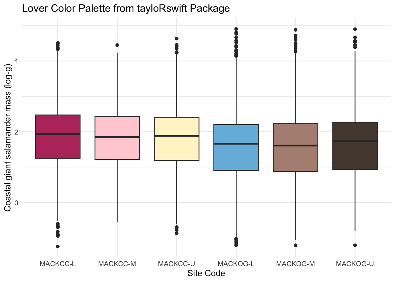
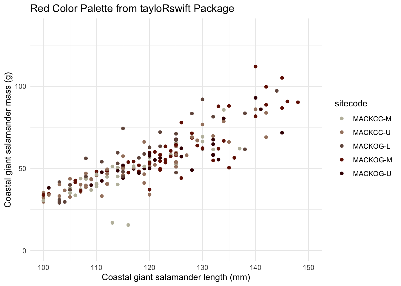
The base plots for this post are from the lterdatasampler package in R, you can learn more about this here: lterdatasampler. I am using data from the Andrews Experimental Forest Long Term Ecological Research Station. I am plotting the weight (log-transformed to make the box plots clearer, in grams) of Giant Coastal Salamanders across study sites in the boxplots, and the length (in mm) and weight Giant Coastal Salamanders in the scatterplots here.

Let’s get coding!

Build base plots & load libraries

Code

library(tidyverse) # data wrangling, and includes ggplot
library(paletteer) # package with a lot of color palettes
library(lterdatasampler) # data I will be using to show off the colors

# base plot
base_plot <- and_vertebrates %>%
  filter(species == "Coastal giant salamander") %>% 
  ggplot(aes(x = sitecode, y = log(weight_g), fill = sitecode)) + # fill the boxes by the variable station
  geom_boxplot() + # make a boxplot
  labs(y = "Coastal giant salamander mass (log-g)", x= "Site Code") +
  guides(fill = FALSE) + # remove legend
  theme_minimal() 

base_plot_scatter <- and_vertebrates %>%
  filter(species == "Coastal giant salamander") %>% 
  filter(sitecode != "MACKCC-L") %>% 
  ggplot(aes(x = length_1_mm, y = weight_g, color = sitecode)) + # color by the variable station
  geom_point() + # make a boxplot
  labs(x = "Coastal giant salamander length (mm)", y= "Coastal giant salamander mass (g)") +
  xlim(100,150) +
  guides(fill = FALSE) + # remove legend
  theme_minimal() 

# base plot
base_plot_twoboxes <- and_vertebrates %>%
  filter(species == "Coastal giant salamander" | species == "Cascade torrent salamander") %>% 
  ggplot(aes(x = species, y = log(weight_g), fill = species)) + # fill the boxes by the variable station
  geom_boxplot() + # make a boxplot
  labs(y = "Mass (log-g)", x= "Species") +
  guides(fill = FALSE) + # remove legend
  theme_minimal()

Taylor Swift Album Covers

tayloRswift is a collection of color palettes made from Taylor Swift’s album covers. You can learn more at the package’s github: asteves tayloRswift github repository.

First, let’s use the direct color palette package, tayloRswift. Next, we will use another package to access these color palettes. Note: in this package, there are 2 functions: one for fill: scale_fill_taylor and one for color: scale_color_taylor.

Code

# install.packages(c("tayloRswift"))
library(tayloRswift) 

# Let's start with the album Lover
base_plot +
  scale_fill_taylor(palette = "lover", guide = "none") +
  ggtitle("Lover Color Palette from tayloRswift Package")

Now, we can try using the paleteer package to load in the palette (no need to install and load library(tayloRswift)). We will use Paleteer to look at the HEX codes for the palette from the album Red (Taylor’s Version, of course).

Code

base_plot_scatter +
  scale_color_manual(values = paletteer_d("tayloRswift::taylorRed")) +
  ggtitle("Red Color Palette from tayloRswift Package")

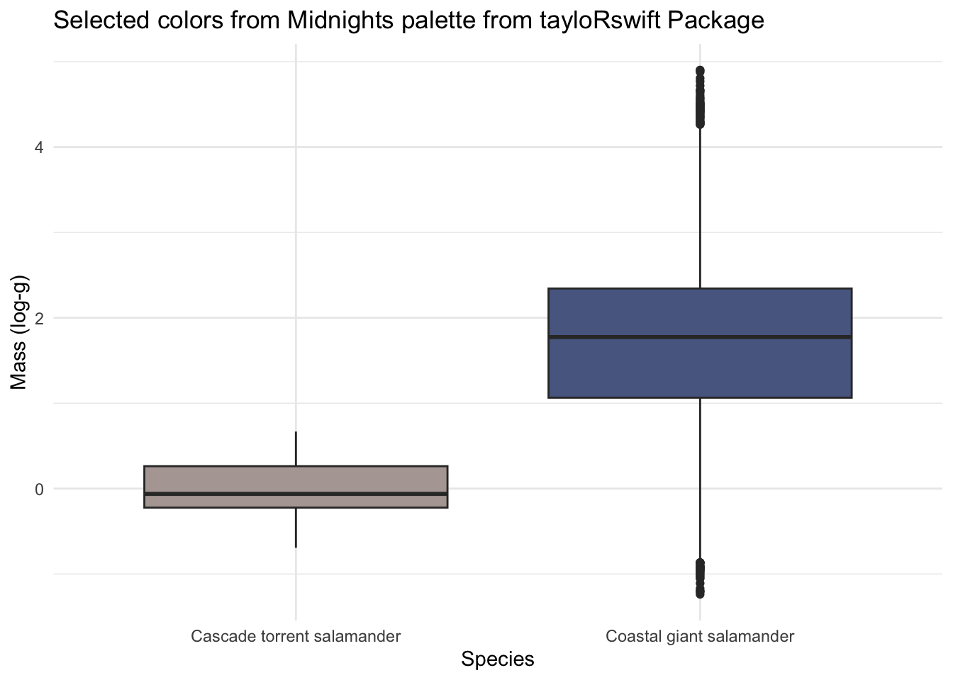
But, what if I want to choose a couple specific colors from the HEX codes? I can use the paleteer_d function to see the HEX codes for each palette

Code

# Let's check out Evermore
paletteer_d("tayloRswift::midnights")

<colors>
#586891FF #8897A4FF #B3A6A3FF #2B152CFF #F1F3F2FF

Code

# Let's say I only want the two of the colors, I can make a new object with the HEX codes output above

my_colors <- c("#B3A6A3FF", "#586891FF")

# Now I can specify these as the colors in my plot
base_plot_twoboxes +
  scale_fill_manual(values = my_colors) +
  ggtitle("Selected colors from Midnights palette from tayloRswift Package")

La Croix Colors

You can learn more at the package’s github: johannesbjork LaCroixColoR github repository

Code

# Let's start with Pamplemousse

# see the hex codes
paletteer::paletteer_d("LaCroixColoR::Pamplemousse")

<colors>
#EA7580FF #F6A1A5FF #F8CD9CFF #1BB6AFFF #088BBEFF #172869FF

Code

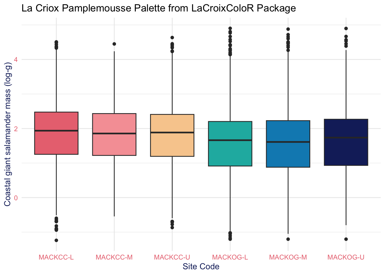
base_plot +
  paletteer::scale_fill_paletteer_d("LaCroixColoR::Pamplemousse") + # NOTE: fill for the boxplot
  ggtitle("La Criox Pamplemousse Palette from LaCroixColoR Package") +
  
  # for fun, let's make the axes text the colors too
  theme(axis.title = element_text(color = "#172869FF"),
        axis.text = element_text(color = "#EA7580FF"))

Code

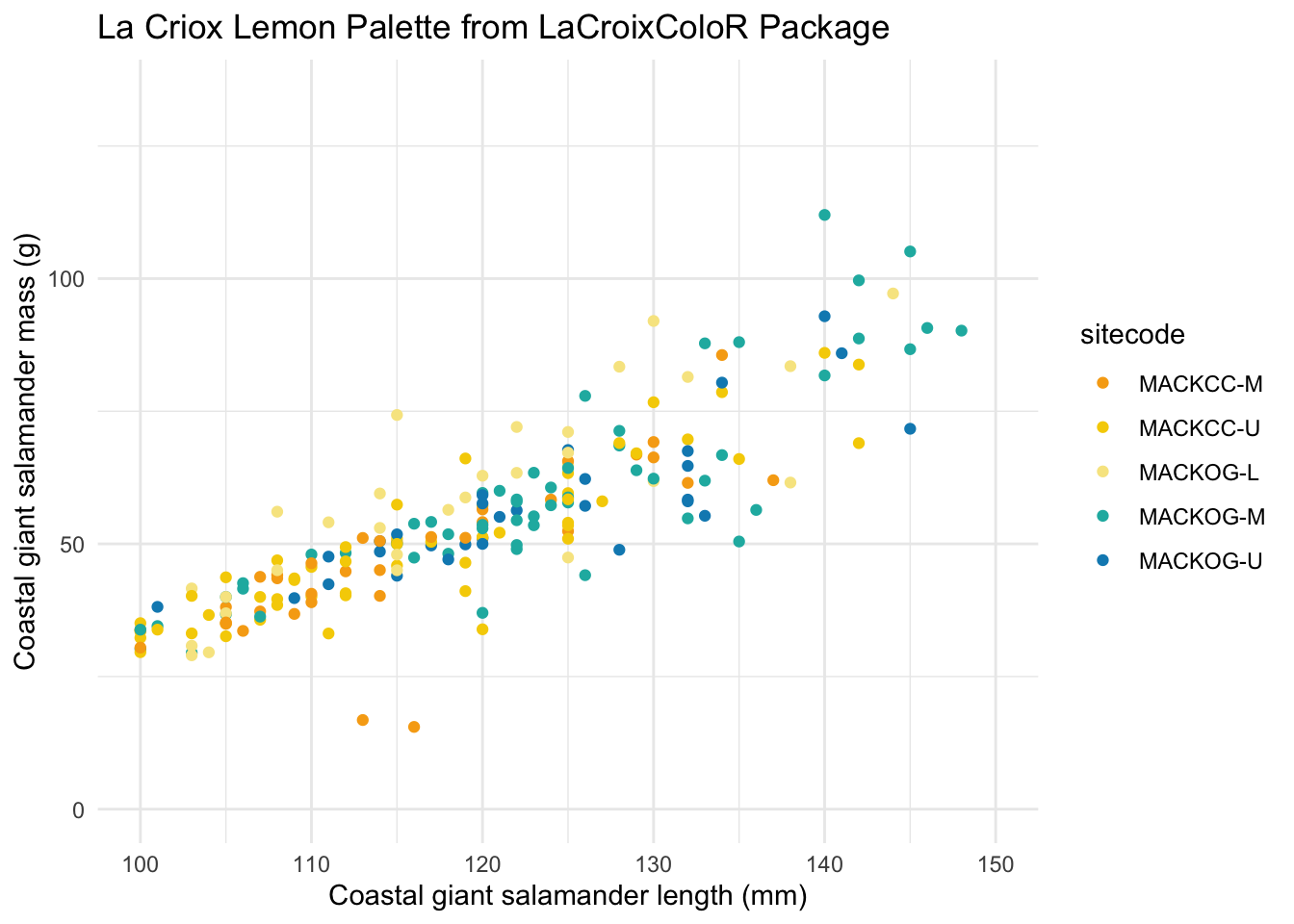
# Now let's do Lemon with a scatterplot

# see the hex codes
paletteer::paletteer_d("LaCroixColoR::Lemon")

<colors>
#F7AA14FF #F5D000FF #F7E690FF #1BB6AFFF #088BBEFF #172869FF

Code

base_plot_scatter +
  paletteer::scale_color_paletteer_d("LaCroixColoR::Lemon") + # NOTE: color for the points
  ggtitle("La Criox Lemon Palette from LaCroixColoR Package")

National Parks Colors

These color palettes come from National Parks posters. You can learn more at the package’s github: katiejolly’s Nationalparkcolors github repository

National Park posters and images

Code

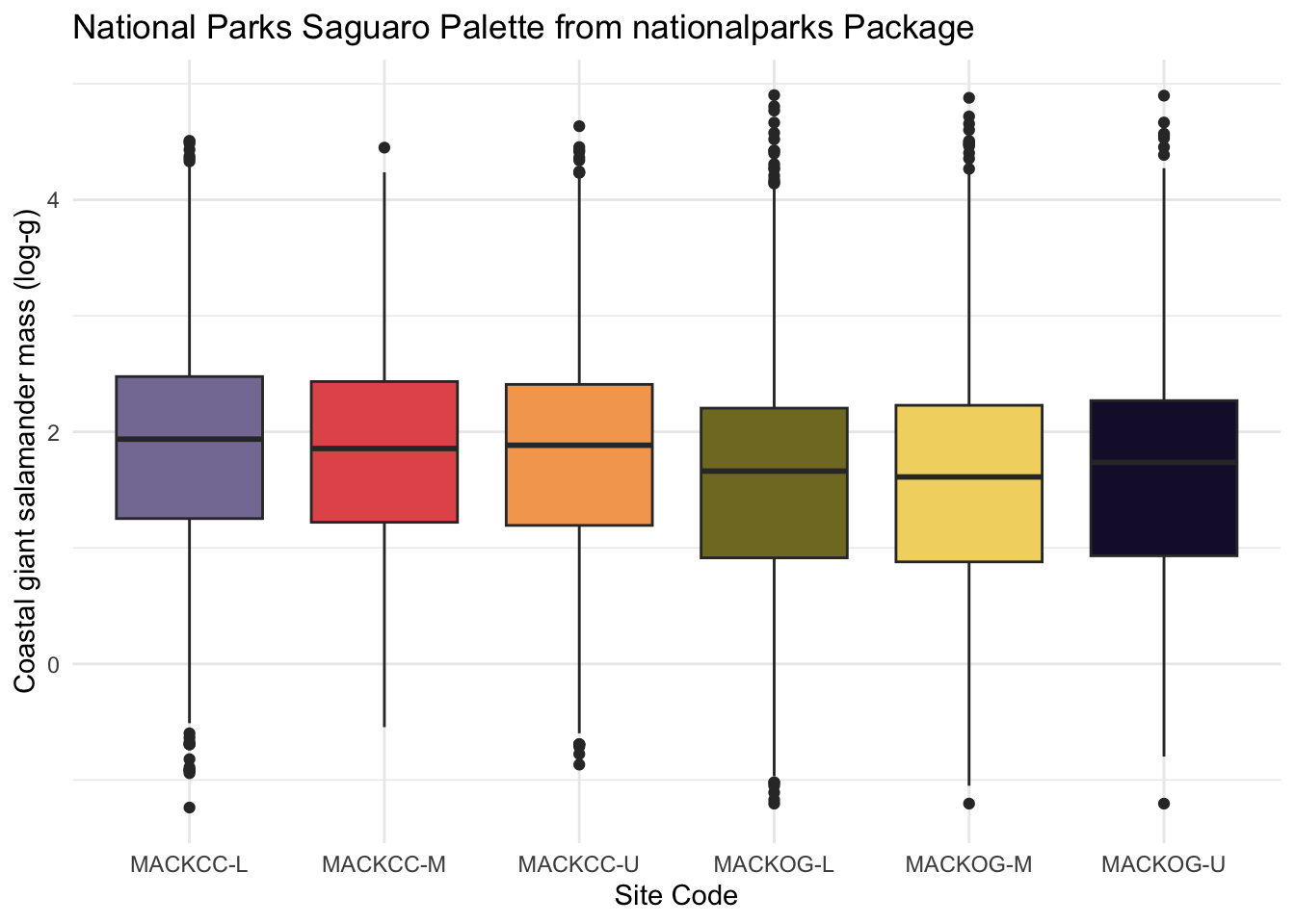
# Let's start with the original package
#devtools::install_github("katiejolly/nationalparkcolors") #uncomment to install
library(nationalparkcolors)

# see the palette
# park_palette("Saguaro")

# build the palette
pal <- park_palette("Saguaro")

base_plot +
  scale_fill_manual(values = pal) +
  ggtitle("National Parks Saguaro Palette from nationalparks Package")

Code

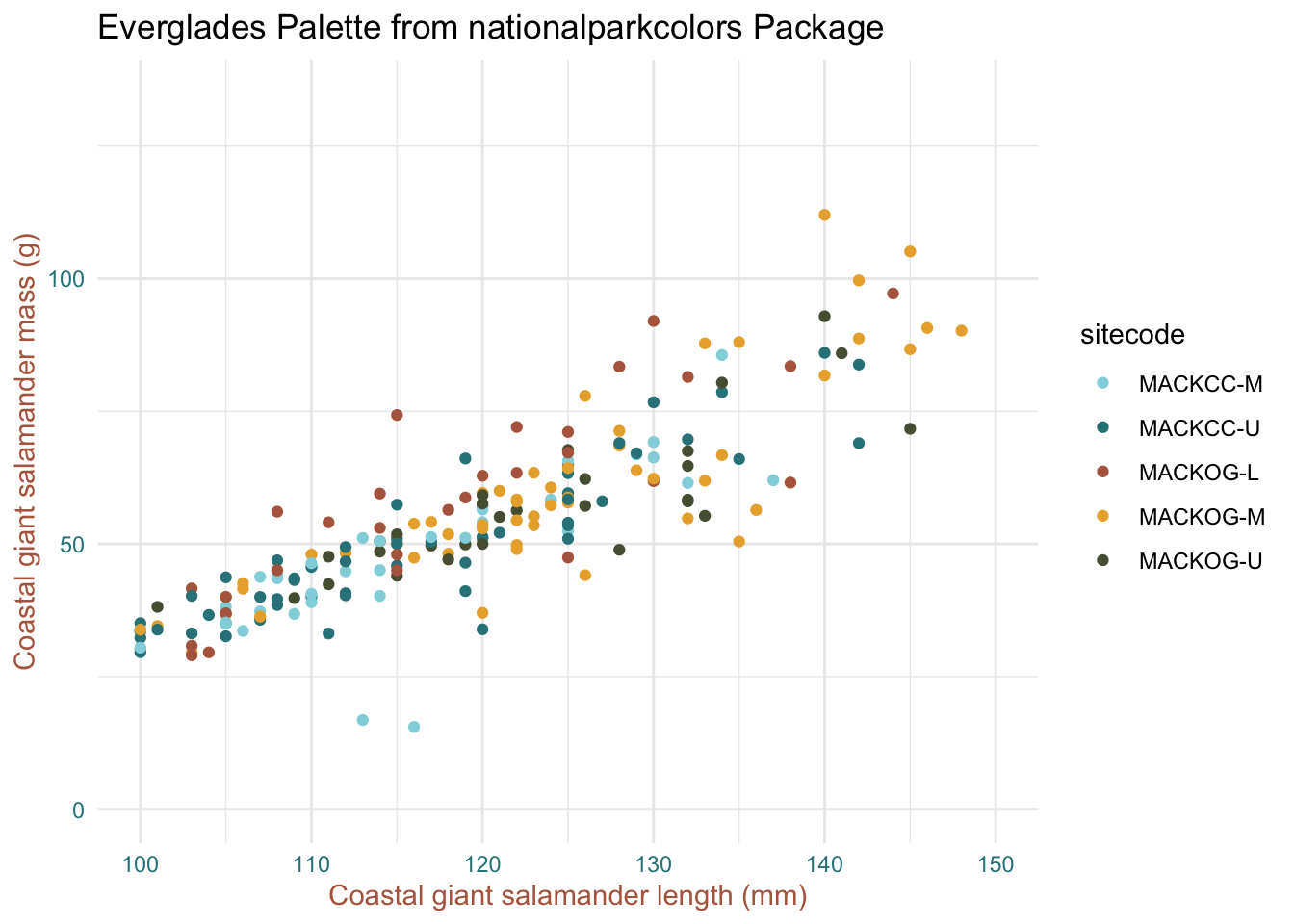
# Now let's do Everglades with paleteer with a scatterplot

# see the hex codes
paletteer::paletteer_d("nationalparkcolors::Everglades")

<colors>
#91D5DEFF #2E8289FF #B4674EFF #EAAE37FF #565F41FF

Code

base_plot_scatter +
  paletteer::scale_color_paletteer_d("nationalparkcolors::Everglades") + # NOTE: color for the points
  ggtitle("Everglades Palette from nationalparkcolors Package") +

  # for fun, let's make the axes text the colors too
  theme(axis.title = element_text(color = "#B4674EFF"),
        axis.text = element_text(color = "#2E8289FF"))

Resources

Sam Csik’s color lecture from her Data Visualization & Communication course in the Masters of Environmental Data Science program at UC Santa Barbara.
An Bui’s Data Visualization Workshop from her Stastics for Environmental Studies Course in the Environmental Studies program at UC Santa Barbara.