Aquaculture Area Analysis

Geospatial analysis of suitable habitat for marine aquaculture

Author

Affiliation

Caitlin Nordheim-Maestas

MEDS coursework at UC Santa Barbara

Research Question & Background

Research Question: Which areas along the U.S. West Coast should be prioritized for marine aquaculture development, based on habitat suitability for multiple commercially important species?

Background

In an era where we are facing an increasing global human population alongside historic losses of biodiversity and overfishing it is vital to focus on sustainable ways to feed our world. Marine aquaculture, especially offshore marine aquaculture (Froehlich et al. 2017), poses a promising future for a more sustainable method of obtaining enough animal protein to meet global demand for animal protein (Gentry et al 2017). First, it is vital to identify what areas to target for the development of marine aquaculture, but this will likely be species-specific, as different species’ physiologies will determine what areas in the ocean are suitable for them. I will focus on determining the suitable area for different species based on their depth tolerance and temperature tolerance, first with oysters, then in a more generalized workflow that allows for the exploration of other marine species.

Moreover, I will demonstrate the utility of the generalized function in R to visualize the areas that are suitable for Red Urchin. Sea urchin aquaculture would be widely applicable for society, as sea urchins are not only harvested for their uni and roe for consumption, but they also contain molecules of pharmaceutical importance for ocular disease investigation, and for biologically active food development (Rubilar & Cardozo 2021).

Data description

I am using Sea Surface Temperature (SST) and Bathymetry data from the ocean off the West Coast of the USA to calculate the suitable habitat in each of the exclusive economic zones (EEZ) in the area for different marine species of aquaculture interest. Exclusive economic zones are the marine area off the coast of an area where the rights to the area’s resources and exploration belong to the owner of that geographic zone.

The SST data was generated from the NOAA Coral Reef Watch 5km Daily Global Satellite Sea Surface Temperature Anomaly, version 3.1, for the years 2008-2012. This is raster data, and each year is a separate raster file, so I averaged the SST for each point across the four years and converted to Celsius.

The Bathymetry data was obtained using General Bathymetric Chart of the Oceans (GEBCO), for the area west of the USA. This is also raster data, all in a single raster file, showing the depth across the geographic area.

In order to determine habitat suitability for certain organisms of aquaculture importance, I used SeaLifeBase to gather the minimum and maximum temperature and depth the species can survive at, which are input into analysis. Note that this data was not imported like the other data sources, but rather, the values discovered in the database are manually input into the workflow for each species.

Then, I use the exclusive economic zone (EEZ) data, obtained through Marineregions.org, to calculate the suitable area for the species in each of the zones in order to compare across zones. This is vector data showing the boundaries of the EEZ’s in this area.

Analysis

Plan

The goal of this work is to create a workflow that can be generalized to any marine species in this geographic areas (in the exclusive economic zones off the West coast of the USA). Thus, I will first walk through the building of the workflow (Part A) for one organism type, oysters. Then in Part B, I will incorporate all of the aspects of the analysis into one function that can work for any species, demonstrating this on Red Urchin.

In Part A, I will (1) import and clean the data for downstream analysis, (2) Determine and map the suitable locations based on SST and depth for a a species, (3) calculate the suitable area per exclusive economic zone, and (4) build a map of the habitable area per EEZ.

In Part B, I will take the workflow from Part A and turn it into a single function, that can take in temperature and depth tolerance data for any species, and output a map with the habitable area per exclusive economic zone in this geographic region. I will first demonstrate that the results are the same using the function for oysters, then will use the function on Red Urchin.

Part A

A.1: Import & clean data

Here, I read in the data, calculate the average sea surface temperature (and convert to Celsius), ensure the bathymetry raster matches the coordinate reference system, extent, and resolution of the SST, and ensure the exclusive economic zone data matches the crs.

Code

# load libraries 
library(tidyverse) # data wrangling
library(janitor) # data wrangling
library(sf) # for spatial data
library(tmap) # for pretty maps
library(here) # file pathing
library(viridisLite) # colors
library(patchwork) # combine plots
library(stars) # rasters
library(terra) # rasters

#..................Sea Surface Temp (SST) Data...................
# read in each raster, one per year
sst_2008 <- rast(here::here("blog", "aquaculture-area-analysis", "data", "average_annual_sst_2008.tif")) 
sst_2009 <- rast(here("blog", "aquaculture-area-analysis", "data", "average_annual_sst_2009.tif"))
sst_2010 <- rast(here("blog", "aquaculture-area-analysis", "data", "average_annual_sst_2010.tif"))
sst_2011 <- rast(here("blog", "aquaculture-area-analysis", "data", "average_annual_sst_2011.tif"))
sst_2012 <- rast(here("blog", "aquaculture-area-analysis", "data", "average_annual_sst_2012.tif"))

# combine SST rasters into a raster stack
sst <- c(sst_2008, 
         sst_2009, 
         sst_2010, 
         sst_2011, 
         sst_2012)

# assign names to each raster layer
names(sst) <- c("2008", 
         "2009",
         "2010",
         "2011",
         "2012")

# local algebra to find the mean sst for each spot
sst_mean <- mean(sst, na.rm = TRUE)

# global algebra to subtract 273.15 to convert from from Kelvin to Celsius
sst_c <- sst_mean - 273.15

#........................Bathymetry Data.........................
# read in bathymetry raster
bath <- rast(here("blog", "aquaculture-area-analysis", "data", "depth.tif"))

# SAME CRS: data check: ensure same crs and reporject if it is not
if(crs(bath) == crs(sst_c)) {
 # print("coordinate reference systems match") # uncomment this for messages to print
} else{
  bath <- project(bath, sst_c) 
}

# SAME EXTENT: crop depth raster to match the extent of the SST raster
# crop bathymetry raster to extent of sst_c
bath_crop <- crop(bath, sst_c)

# SAME RESOLUTION: resample to ensure the resolutions match
# using the nearest neighbor approach
bath_final <- resample(bath_crop, y = sst_c, 
                          method = "near") # for nearest neighbor

#...............Exclusive Economic Zone (EEZ) Data...............
eez <- st_read(here("blog", "aquaculture-area-analysis", "data", "wc_regions_clean.shp"), 
               quiet = TRUE) # no message output

# crs match
if(crs(eez) == crs(sst_c)) {
 # print("coordinate reference systems match") # uncomment this for messages to print
} else{
  eez <- st_transform(eez, crs = st_crs(sst_c))
}

A.2: Suitable locations for oysters

Now I will find suitable locations for marine aquaculture in terms of both SST and depth. Here, I will use oysters as an example organism, and they can only exist between 11-30 degrees C and -70 through 0 meters below sea level.

I will build matrices for temperature sst_matrix, and the depth bath_matrix, which include all values from -Infinity to +Infinity, specifying if they are habitable for the species with a 1 or uninhabitable with a 0. Next, I will reclassify the original rasters with whether each area is suitable using its matrix.

Code

# build matrix of habitable (1) and uninhabitable (0) temperatures
sst_matrix <- matrix(c(-Inf, 11, 0, # temperature too low
                        11, 30, 1, # habitable temperatures
                        30, Inf, 0), # temperature too high
                        ncol = 3, byrow = TRUE)

# use reclassification matrix to reclassify temperature raster to suitable areas according to temp
sst_rcl <- classify(sst_c, rcl = sst_matrix)

# build matrix of habitable (1) and uninhabitable (0) depths
bath_matrix <- matrix(c(-Inf, -70, 0, # depth too low
                        -70, 0, 1, # habitable depth
                        0, Inf, 0), # depth too high 
                        ncol = 3, byrow = TRUE)

# use reclassification matrix to reclassify bathymetry raster to suitable areas according to depth
bath_rcl <- classify(bath_final, rcl = bath_matrix)

The SST and depth rasters now identify the suitability of locations as 0 or 1. To find locations that have both suitable temperature and depth, I can use a map algebra trick and mulitply the rasters together. This works because anything multiplied by 0 equals 0 and anything multiplied by 1 equals itself. Thus, any areas that are uninhabitable due to temperature or depth or both will be 0, and only areas where both are habitable (multiplying 1*1) will end up as 1, also known as habitable area.

Code

# determine the suitable cells using the reclassified sst and depth multiplying them
suitable_cells <- sst_rcl * bath_rcl

# make 0's NA
suitable_cells[suitable_cells == 0] <- NA

A.3: Area per EEZ

Now that we know which areas off the West Coast of the USA are habitable for our species of interest, here oysters, based on SST and depth, we can calculate how much area is habitable in each exclusive economic zone (EEZ), to allow for comparison across zones. This comparison can lead to management decisions about which zones are the best to explore marine aquaculture development for a specific species of interest.

Code

# crop suitable cells to eez
suitable_cropped <- crop(suitable_cells, eez)

# rasterize eez
eez_rast <- rasterize(eez, suitable_cropped, field = "area_km2")

# compute the area covered by individual raster cells in km
suitable_cropped <- terra::cellSize(suitable_cropped, # Compute the area covered by individual raster cells
                             mask=TRUE, # If TRUE, cells that are NA remain NA in the output
                             lyrs=FALSE, # If TRUE and mask=TRUE, the output has the same number of layers as input
                             unit="km") # report the cell area in km

# use zonal stats to get the sum of the area in each eez
zones_suitarea <- terra::zonal(suitable_cropped, # x: SpatRaster
                               eez_rast, # y: needs to be terra object
                               fun = "sum", # sum up the area
                               na.rm = TRUE) # remember to remove NA's!

# update the column names from the initial dataframe of the eez
zones_clean <- cbind(eez, zones_suitarea) %>%  
  # clean dataframe for ease of use
  dplyr::select(rgn, area_km2, area) %>% # select columns I care about
  rename("suitable_area" = "area") # rename to something prettier

A.4: Build map

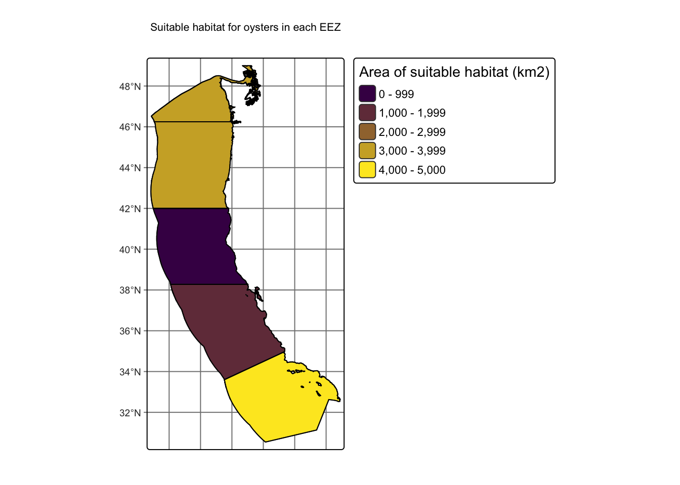
I will now build a map of the amount of habitable area there is for this species (oysters) per exclusive economic zone. This map will visualize the results of the amount of habitable area per EEZ, and allow for easy comparisons across the EEZ to select the zone with the most habitable area. It can be used to explore latitudinal patterns in the habitability for a specific species. Importantly, building a map will allow for easy comparison across different species, when multiple maps are made.

Code

map <- tm_shape(zones_clean) + # vector data, use tmshape. 
    tm_graticules() + # add graticules at this layer
 
# next layer: fill by area of suitable habitat
  tm_polygons(fill = "suitable_area", # column name with the values
  # specify the color scale, using viridis because it is colorblind friendly
              fill.scale = tm_scale(values =  viridis(2)), 
              fill.legend = tm_legend(title = "Area of suitable habitat (km2)", 
                                      position = tm_pos_out("right"))) +
  
 # next layer: show the outlines of the zones clearly
  tm_borders(col = "black") + # borders of the counties

# add map elements
  tm_title(text = "Suitable habitat for oysters in each EEZ") 

map

Part B: Generalizable workflow

Now that I know that the workflow functions, I am going to take all of the steps done prior and put them into one function that can intake information for any species and output the same map for that species. This allows for easy comparison across species which will allow for us to determine which EEZ’s are best across multiple species and help inform marine aquaculture management. Functionally, it will save a lot of space to only need to input a species’ information rather than repeating the whole workflow. Moreover, it will maximize reproducibility so other can easily use this tool, and minimize the change of small errors in coding that may arise when copy and pasting lots of code in the absence of a single function.

Code

suitable_habitat <- function(bath, # bathymetry raster
                             eez, # eez spatial dataframe
                             sst_c, # raster of sea surface temp; 
                             #with mean sst for the time period you want
                             min_sst, # string with the minimum temp in C
                             max_sst, # string with the max temp in C
                             min_depth_m, # string with the minimum depth in m
                             max_depth_m, # string with the maximum temp in m
                             species_name) # string with species name
  {
#...............STEP 1: Bathymetry raster cleaning...............
  # SAME CRS: project bath to sst_c
       bath <- project(bath, sst_c) 
  # Now crop to same extent: crop bathymetry raster to extent of sst_c
    bath_crop <- crop(bath, sst_c)
  # now ensure in same resolution as sst by resampling, use nearest neighbor
    bath_final <- resample(bath_crop, y = sst_c, 
                          method = "near") # for nearest neighbor

#........STEP 2: build a suitable depth and temp raster.......
    # build a matrix for reclassifying sst
      sst_matrix <- matrix(c(-Inf, min_sst, 0, # uninhabitable
                        min_sst, max_sst, 1, # habitable
                        max_sst, Inf, 0), # uninhabitable
                        ncol = 3, byrow = TRUE)
    # use reclassification matrix to reclassify elevation raster
    sst_rcl <- classify(sst_c, rcl = sst_matrix)
  # build a matrix for reclassifying bathymetry
    bath_matrix <- matrix(c(-Inf, max_depth_m, 0, # uninhabitable
                        max_depth_m, min_depth_m, 1, # habitable
                        min_depth_m, Inf, 0), # uninhabitable
                        ncol = 3, byrow = TRUE)
    # use reclassification matrix to reclassify elevation raster
    bath_rcl <- classify(bath_final, rcl = bath_matrix)
    # determine the suitable cells using the reclassified sst and depth multiplying
    # call the output suitable_cells
    suitable_cells <- sst_rcl * bath_rcl
    # make 0's NA
    suitable_cells[suitable_cells == 0] <- NA

#..........STEP 3: incorporate exclusive economic zones..........    
    # crop suitable cells to eez
    suitable_cropped <- crop(suitable_cells, eez)
    # rasterize eez
    eez_rast <- rasterize(eez, suitable_cropped, field = "area_km2")
    # compute the area covered by individual raster cells
    suitable_cropped <- cellSize(suitable_cropped, mask=TRUE, lyrs=FALSE, unit="km")
    # use zonal stats
    zones_suitarea <- terra::zonal(suitable_cropped, # x: SpatRaster
                               eez_rast, # y: needs to be terra object
                               fun = "sum", # sum up the area
                               na.rm = TRUE) 
    # update the column names from the initial sf df
     zones <- cbind(eez, zones_suitarea) %>% 
     # clean the dataframe
       dplyr::select(rgn, area_km2, area) %>% # select columns I care about
       rename("suitable_area" = "area") # rename to something prettier
    
#........................STEP 4: Mapping.........................
 map <- tm_shape(zones) + # vector data, use tmshape. 
    tm_graticules() + # add graticules at this layer
 
# next layer: fill by area of suitable habitat
  tm_polygons(fill = "suitable_area", # column name with the values
  # specify the color scale, using viridis because it is colorblind friendly
              fill.scale = tm_scale(values =  viridis(2)), 
              fill.legend = tm_legend(title = "Area of suitable habitat (km2)", 
                                      position = tm_pos_out("right"))) +
  
 # next layer: show the outlines of the zones clearly
  tm_borders(col = "black") + # borders of the counties

# add map elements: title with species name
  tm_title(text = paste0("Suitable habitat for ", species_name))

 # assign name to map
  assign(paste0(species_name, "_map"), map, envir = .GlobalEnv)
}

Results

Use function on Oysters to ensure same output

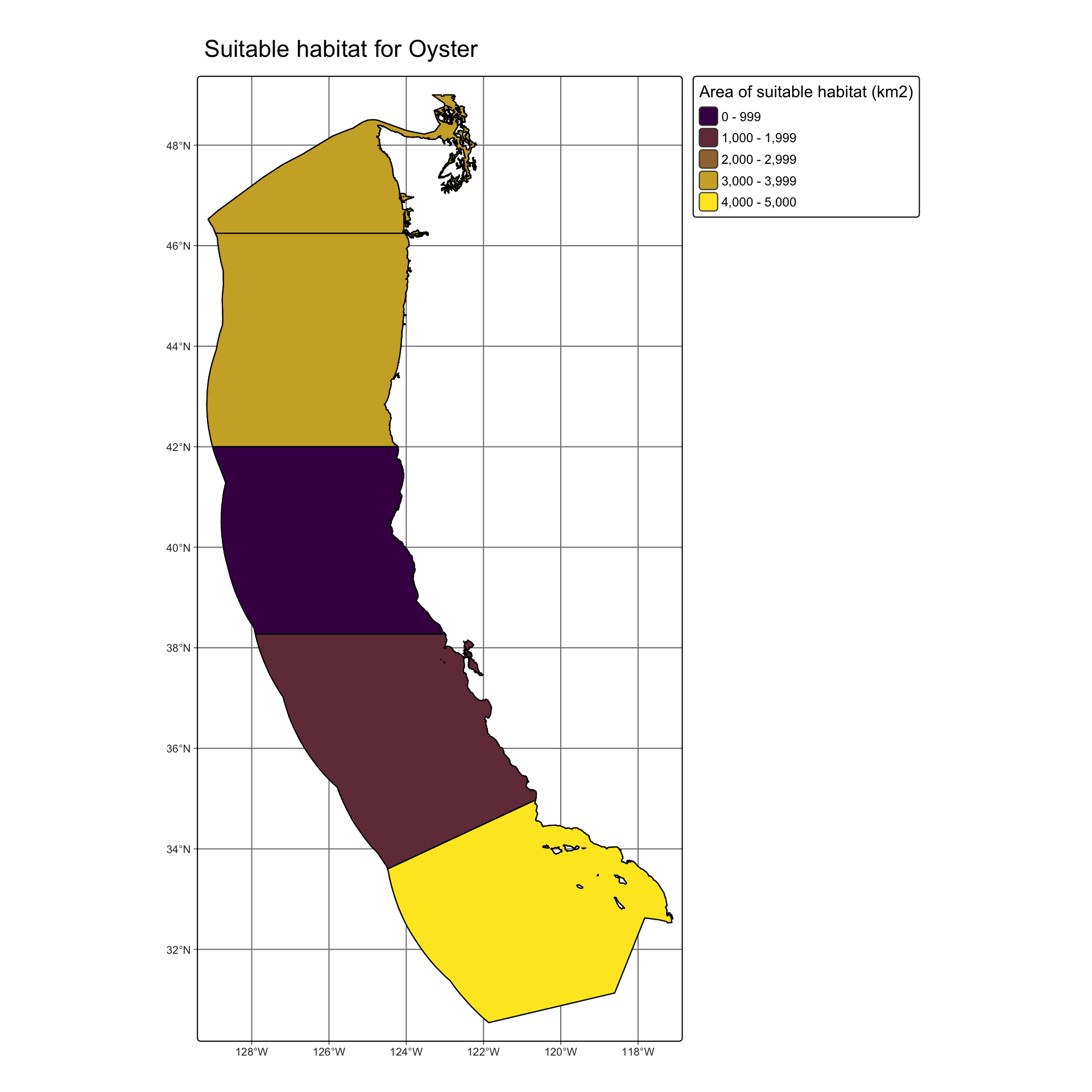
Here I can demonstrate that the function is working by using the same inputs for oysters above and comparing the output.

Code

oyster_output <- suitable_habitat(bath = bath_final,
                  eez = eez, # eez spatial dataframe
                  sst_c = sst_c, # raster of sea surface temp
                  min_sst = 11, # string with the minimum temp in C
                  max_sst = 30, # string with the max temp in C
                  min_depth_m = 0, # string with the minimum depth in m
                  max_depth_m = -70, # string with the maximum temp in m
                  species_name = "Oyster") # string with species name)
oyster_output

Figure 1. Map of Exclusive Economic Zones off the West Coast of the USA colored by the amount of suitable habitat area for oysters in square kilometers. The suitable habitat was calculated using the thermal and depth limits of the species.

Since we see the same output, we can trust the function works and use it for other species!

Using function on new species: Red Urchin

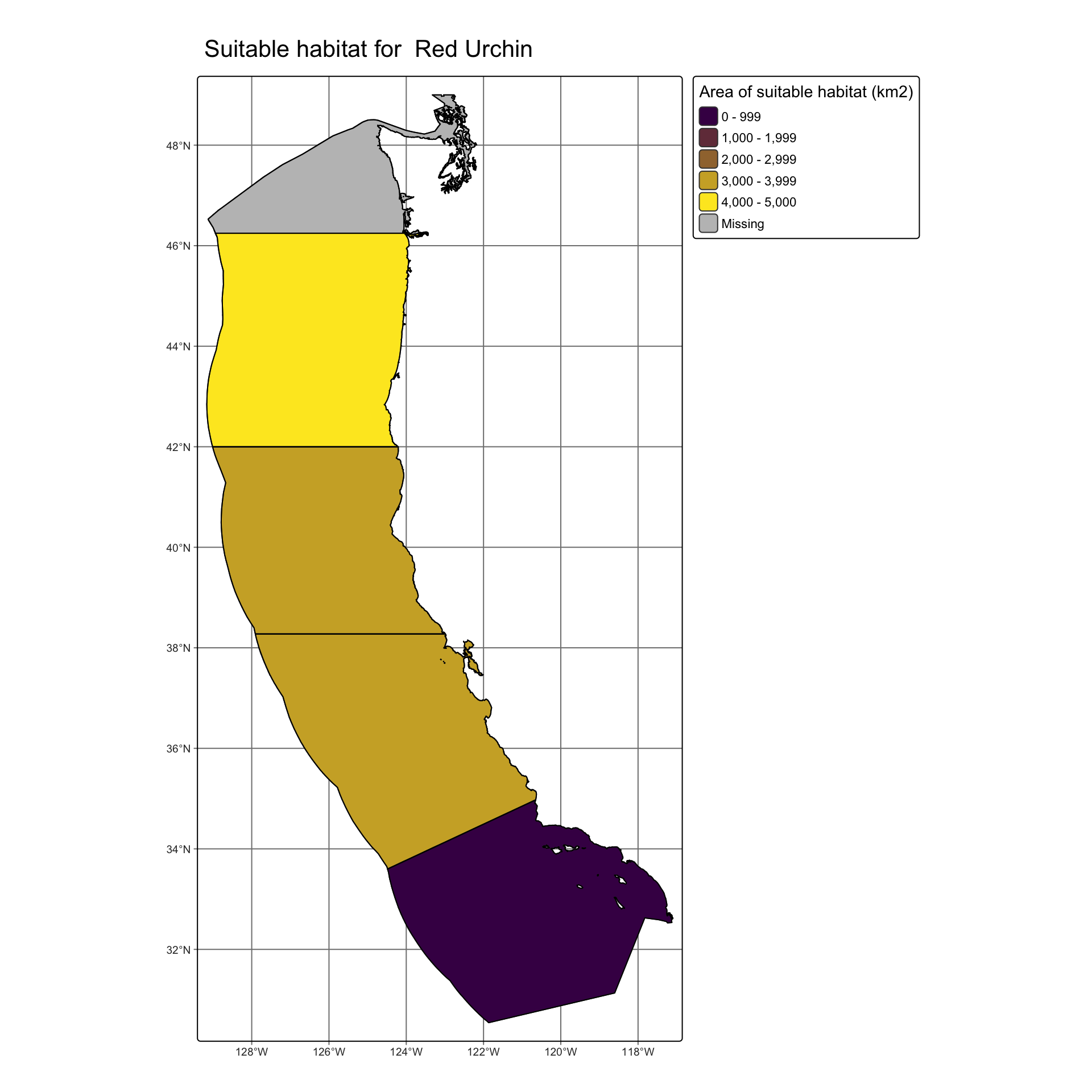
Now, I will use the workflow on a new species, Red Urchin, which will allow me to visualize the best EEZ areas to investigate for marine aquaculture for Red Urchin, and to compare this map with the map of oysters.

Code

# set parms for the function for the red sea urchin
min_sst <- 4.1
max_sst <- 10.7
min_depth_m <- 0
max_depth_m <- -125
species_name <- " Red Urchin"

# run my function
urchin_output <- suitable_habitat(bath = bath_final,
                  eez = eez, # eez spatial dataframe
                  sst_c = sst_c, # raster of sea surface temp
                  min_sst = min_sst, # string with the minimum temp in C
                  max_sst = max_sst, # string with the max temp in C
                  min_depth_m = min_depth_m, # string with the minimum depth in m
                  max_depth_m = max_depth_m, # string with the maximum temp in m
                  species_name = species_name) # string with species name)
urchin_output

Figure 2. Map of Exclusive Economic Zones off the West Coast of the USA colored by the amount of suitable habitat area for red urchin (Mesocentrotus franciscanus) in square kilometers. The suitable habitat was calculated using the thermal and depth limits of the species.

Discussion

Overall, I found that there is a vast amount of area suitable off of the West Coast of the USA for oysters (Figure 1) and for Red Sea Urchin (Figure 2), where each species has exclusive economic zones with over 4,000 square kilometers of suitable area. This work also highlights the importance of making species-specific investigations into where to invest in marine aquaculture, as the oysters had more suitable area in South, but the South-most EEZ was the worst of the options for Red Urchin, which would have more area in the North.

It is important to note that this analysis does not take all important aspects of habitability for the species, or feasibility of using the area for aquaculture. This analysis and tool should be used as a first-step to determine where to look deeper into the feasibility of building marine aquaculture for a specific species. For example, an example of a future iteration of this tool would exclude areas with low phytoplanktonic food availability when considering bivalves (Gentry et al 2017), and exclude areas that are off-limits for aquaculture, like marine protected areas (MPAs), shipping lanes, and oil rigs, as done in Gentry et al 2017. This could be incorporated into this workflow by reading in maps of the MPAs, shipping areas, and areas owned by oil rigs, and subtracting them from the suitable areas.

Works Cited

Journal articles

Froehlich, Halley E., Alexandra Smith, Rebecca R. Gentry, and Benjamin S. Halpern. “Offshore aquaculture: I know it when I see it.” Frontiers in Marine Science 4 (2017): 154.

Gentry, Rebecca R., Halley E. Froehlich, Dietmar Grimm, Peter Kareiva, Michael Parke, Michael Rust, Steven D. Gaines, and Benjamin S. Halpern. “Mapping the global potential for marine aquaculture.” Nature ecology & evolution 1, no. 9 (2017): 1317-1324.

Rubilar, Tamara, and Dana Cardozo. “Blue growth: sea urchin sustainable aquaculture, innovative approaches.” Revista de Biología Tropical 69 (2021): 474-486.

Data citations

SST

NOAA Coral Reef Watch. NOAA Coral Reef Watch Version 3.1 Daily 5km Satellite Regional Virtual Station Time Series Data for West Coast of USA, 2008 - 2012r. College Park, Maryland, USA: NOAA Coral Reef Watch. Data set accessed at https://coralreefwatch.noaa.gov/product/vs/data.php.

Bathymetry

GEBCO Compilation Group (2022) GEBCO_2022 Grid (doi:10.5285/e0f0bb80-ab44-2739-e053-6c86abc0289c).

EEZ

Flanders Marine Institute (2025): MarineRegions.org. Available online at www.marineregions.org. Consulted on 2025-11-25.

SeaLifeBase

Palomares, M.L.D. and D. Pauly. Editors. 2025. SeaLifeBase. World Wide Web electronic publication. www.sealifebase.org, version (04/2025).